Copy page

• Copy page
• View source

Applied Nuclear Data Assimilation using GLLS

This example demonstrates the use of the Generalized Least Squares (GLLS) method to combine experimental benchmark data with prior nuclear data covariance information, producing a posterior set of cross section, nu-bar, and prompt fission spectrum adjustments. It then walks through the full verification path: exporting those adjustments directly onto existing ACE files with AssimilationSuite.to_ace_direct, and confirming that the resulting pointwise ACE perturbation matches the multigroup adjustment GLLS predicted.

Benchmarks:

• HMF001

• HMF002-001

Application:

• HMF002-002

1. Setup and posterior calculation

We use andalus for the assimilation and ACE perturbation logic, pandas to interact with the adjustment data, and matplotlib for visualization. It is assumed the reader is familiar with creating a posterior from the other example notebooks. Therefore, a couple of steps are skipped.

import matplotlib.pyplot as plt

import andalus

plt.style.use("ggplot")

assimilation_suite = andalus.AssimilationSuite.from_yaml("config.yaml")
posterior_suite = assimilation_suite.glls()

Reading ../data/hmf001.ser_res.m
WARNING:  SERPENT Serpent 2.2.1 found in ../data/hmf001.ser_res.m, but version 2.1.31 is defined in settings
WARNING:    Attempting to read anyway. Please report strange behaviors/failures to developers.
  - done
Reading ../data/hmf001.ser_sens0.m
  - done
Reading ../data/hmf001.ser_det0.m
  - done
Reading ../data/hmf002-001.ser_res.m
WARNING:  SERPENT Serpent 2.2.1 found in ../data/hmf002-001.ser_res.m, but version 2.1.31 is defined in settings
WARNING:    Attempting to read anyway. Please report strange behaviors/failures to developers.
  - done
Reading ../data/hmf002-001.ser_sens0.m
  - done
Reading ../data/hmf002-002.ser_res.m
WARNING:  SERPENT Serpent 2.2.1 found in ../data/hmf002-002.ser_res.m, but version 2.1.31 is defined in settings
WARNING:    Attempting to read anyway. Please report strange behaviors/failures to developers.
  - done
Reading ../data/hmf002-002.ser_sens0.m
  - done

Performing GLLS update on the assimilation suite...
    Number of benchmarks included in GLLS: 2
    Prior chi-squared with nuclear data: 0.0095
    Prior chi-squared without nuclear data: 1.3981
    Posterior chi-squared with nuclear data: 0.0002
    Posterior chi-squared without nuclear data: 0.0004

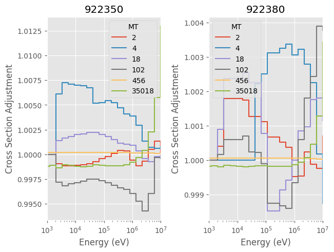
2. Cross-Section Adjustments by nuclide

The posterior calculated values in the previous plot are produced by an underlying set of multigroup relative adjustments to each isotope’s reactions, stored in posterior_suite.xs_adjustment. Plotting these directly shows which reactions GLLS moved, by how much, and in which energy range.

posterior_suite.xs_adjustment

ZAI     MT     E_min_eV      E_max_eV
922350  2      1.000000e-05  1.000000e-01   -6.999980e-08
               1.000000e-01  5.400000e-01   -7.257689e-08
               5.400000e-01  4.000000e+00   -8.003348e-08
               4.000000e+00  8.315290e+00   -6.732921e-08
               8.315290e+00  1.370960e+01   -3.360391e-08
                                                 ...
922380  35018  1.353350e+06  2.231300e+06   -6.864650e-05
               2.231300e+06  3.678790e+06    7.505350e-05
               3.678790e+06  6.065310e+06    4.516108e-04
               6.065310e+06  1.000000e+07    1.283729e-03
               1.000000e+07  1.964030e+07    3.430290e-03
Length: 396, dtype: float64

fig, axs = plt.subplots(1, 2, layout="constrained")

e_low = posterior_suite.xs_adjustment.loc[922350].loc[18].index.get_level_values("E_min_eV")

for i, zai in enumerate([922350, 922380]):
    ax = axs[i]

    for mt in posterior_suite.xs_adjustment.loc[922350].index.get_level_values("MT").unique():
        ax.step(e_low, posterior_suite.xs_adjustment.loc[zai].loc[[mt]].values + 1, where="post", label=mt)

    ax.set(
        xscale="log",
        xlabel="Energy (eV)",
        ylabel="Cross Section Adjustment",
        xlim=(1e3, 1e7),
        title=zai,
    )

    ax.legend(title="MT")

5. Exporting the Posterior to ACE

The multigroup adjustments above are a linear approximation of how the nuclear data should change to reproduce the benchmark measurements. To verify that approximation without reprocessing the ENDF evaluation through NJOY, AssimilationSuite.to_ace_direct applies the same adjustments directly onto an already-processed ACE file for each isotope, editing the pointwise cross sections, nu-bar, and prompt fission spectrum in place.

MTs are routed automatically: 452/456 (nu-bar) go to ACE.perturb_nu, MT \(\geq\) 35000 (ANDALUS’s MF \(\times\) 1000 + MT chi convention, e.g. 35018 for the prompt fission spectrum of MT=18) go to ACE.perturb_chi, and every other reaction MT goes to ACE.perturb. Source ACE files are located through a Serpent-style xsdata file (test.xsdata); create_xsdata=True also writes one describing the perturbed output, so the posterior library can be used directly in a follow-up Serpent run.

# Only test the methodology for U-235
posterior_suite.xs_adjustment = posterior_suite.xs_adjustment.loc[[922350]]

posterior_suite.to_ace_direct(out_dir="posterior_ace", xsdata_path="../data/test.xsdata", create_xsdata=True)

['posterior_ace\\92235.03c']

!cat posterior_ace/adjusted.xsdata

  92235.03c 92235.03c 1 92235 0 235.0 300 0 92235.03c

6. Verifying the Cross-Section Adjustment

We read back the prior source ACE file and the perturbed posterior ACE file for the same isotope, and compare the pointwise ratio between them to the multigroup adjustment GLLS originally predicted. If to_ace_direct applied the adjustment correctly, the pointwise ACE ratio should step through the same relative change as the GLLS curve at every energy.

zai = 922350

u235_prior = andalus.ace.ACE.read(f"../data/{zai / 10:.0f}.03c")
u235_post = andalus.ace.ACE.read(f"posterior_ace/{zai / 10:.0f}.03c")

mt = 18

fig, ax = plt.subplots(layout="constrained")

prior = u235_prior.reactions[mt]
post = u235_post.reactions[mt]

ratio = post.xs / prior.xs

ax.step(
    posterior_suite.xs_adjustment.loc[zai].loc[mt].index.get_level_values("E_min_eV"),
    posterior_suite.xs_adjustment.loc[zai].loc[mt].values,
    marker="x",
    where="post",
    label="GLLS",
)
ax.plot(prior.energies * 1e6, ratio - 1, label="ACE")

ax.set(xscale="log", xlabel="Energy (eV)", ylabel="Cross Section (barns)", xlim=(1e3, 20e6), title=f"MT {mt}")

ax.legend()

<matplotlib.legend.Legend at 0x2ab2f209d00>

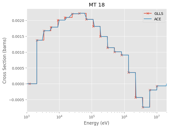
The pointwise ACE ratio follows the GLLS step function closely across the full energy range. This confirms that perturb correctly redistributed the fission adjustment onto U-238’s constituent reactions and that the perturbed ACE file reproduces the same multigroup shift used in the GLLS model, without relying on the linear approximation any further.

7. Verifying the Nu-Bar Adjustment

Nu-bar (the average number of neutrons released per fission) is perturbed independently of the cross sections via ACE.perturb_nu, using MT=456 for prompt nu-bar. We compare the same way: the pointwise ratio of the perturbed to the prior tabulated nu-bar values against the GLLS adjustment for MT=456.

mt = 456

fig, ax = plt.subplots(layout="constrained")

prior = u235_prior.nu["prompt"]
post = u235_post.nu["prompt"]

ratio = post.values / prior.values

ax.step(
    posterior_suite.xs_adjustment.loc[zai].loc[mt].index.get_level_values("E_min_eV"),
    posterior_suite.xs_adjustment.loc[zai].loc[mt].values,
    marker="x",
    where="post",
    label="GLLS",
)
ax.plot(prior.energy * 1e6, ratio - 1, label="ACE")

ax.set(
    xscale="log",
    xlabel="Energy (eV)",
    ylabel="Cross Section (barns)",
    # yscale="log",
    xlim=(1e3, 20e6),
    title="Prompt neutron multiplicity",
)

ax.legend()

<matplotlib.legend.Legend at 0x2ab3e87a540>

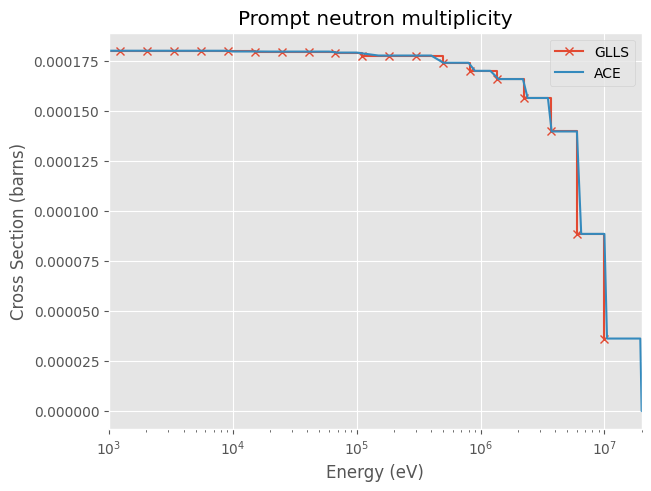
Again, the ACE nu-bar ratio matches the GLLS prediction at every incident energy, confirming that perturb_nu applied the adjustment to the correct tabulated nu-bar table.

8. Verifying the Prompt Fission Spectrum Adjustment

The prompt fission neutron spectrum \(\chi(E_{out})\) is stored per incident energy in the ACE DLW block and perturbed via ACE.perturb_chi under MT=35018. ANDALUS does not yet resolve chi sensitivities by incident energy, so the same outgoing-energy-binned adjustment is applied identically to every incident-energy table; here we inspect one representative table (index 15) and compare its perturbed-to-prior PDF ratio against the GLLS adjustment.

mt = 35018

fig, ax = plt.subplots(layout="constrained")

prior = u235_prior.chi[18].tables[15]
post = u235_post.chi[18].tables[15]

ratio = post.pdf / prior.pdf

ax.step(
    posterior_suite.xs_adjustment.loc[zai].loc[mt].index.get_level_values("E_min_eV"),
    posterior_suite.xs_adjustment.loc[zai].loc[mt].values,
    marker="x",
    where="post",
    label="GLLS",
)
ax.plot(prior.energy_out * 1e6, ratio - 1, label="ACE")

ax.set(
    xscale="log",
    xlabel="Energy (eV)",
    ylabel="Cross Section (barns)",
    xlim=(1e3, 20e6),
    title="Prompt neutron energy spectrum",
)

ax.legend()

<matplotlib.legend.Legend at 0x2ab3ebe50a0>

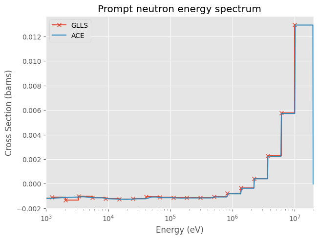
The pointwise chi ratio again follows the GLLS step function, confirming that perturb_chi applied the outgoing-energy adjustment to the prompt fission spectrum correctly. If however, the ACE data does not have an energy point within an energy group, no new energy point is added and the bin is skipped.

Together, the three verification plots show that to_ace_direct reproduces the GLLS posterior at the pointwise ACE level, so the perturbed library can be used directly in a Monte Carlo transport calculation to check the posterior without any further reliance on the linear GLLS approximation.