Visualizing Serpent Sensitivity Profiles
This example demonstrates how to use the andalus package to process and visualize sensitivity profiles generated by the Serpent-2 Monte Carlo neutron transport code. Sensitivity analysis is crucial in nuclear data assimilation to understand how uncertainties in specific cross-sections affect integral parameters like \(k_{\text{eff}}\).
1. Setup and Imports
First, we import matplotlib for figure customization and the andalus core package.
[7]:
import matplotlib.pyplot as plt

import andalus
2. Reading Serpent Output
We use the Sensitivity.from_serpent method to parse the .m file.
In this example, we examine the HMF001 (Godiva) benchmark. We filter the perturbations (pertlist) for specific reaction types (MT) as denoted in the sens0.m output file:
mt 2: Elastic scatteringmt 4: Inelastic scatteringmt 18: Fissionmt 102: Radiative capturenubar prompt: Average number of outgoing prompt neutrons per fissionchi prompt: Outgoing prompt neutron energy distribution
[8]:
file_path = "../data/hmf001.ser_sens0.m"
hmf001 = andalus.Sensitivity.from_serpent(
    sens0_path=file_path, title="HMF001", pertlist=["mt 2 xs", "mt 4 xs", "mt 18 xs", "mt 102 xs"]
)
Reading ../data/hmf001.ser_sens0.m
  - done
3. Plotting Energy-Dependent Sensitivities
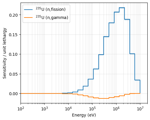
We can now plot the sensitivity profiles for specific isotopes. Below, we focus on U-235 (ZAI 922350) for Fission (MT 18) and Capture (MT 102) reactions.
[9]:
zais = [922350]  # U-235
perts = [18, 102]  # Fission and Capture

fig, ax = plt.subplots(figsize=(5, 4), layout="constrained")

for zai in zais:
    for pert in perts:
        hmf001.plot_sensitivity(zais=[zai], perts=[pert], ax=ax)

ax.set(
    xlim=(1e2, 2e7),
)

plt.show()
C:\Users\dhouben\Documents\andalus\src\andalus\sensitivity.py:230: PerformanceWarning: indexing past lexsort depth may impact performance.
  subset = self.loc[zai, pert]
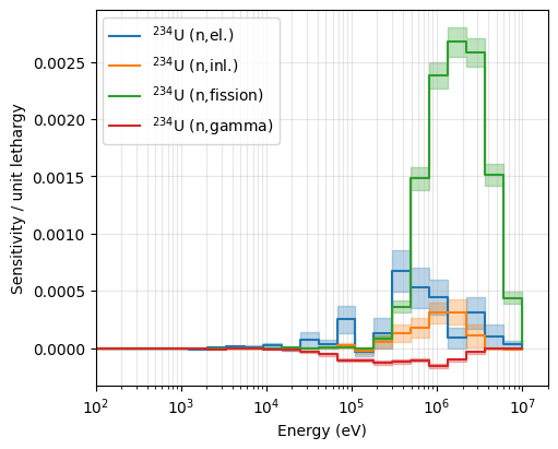
Next, we plot the sensitivity profiles for U-234. As \(k_{\text{eff}}\) is less sensitive to U-234, the sensitivity estimates obtained via Serpent also suffers more from statistical noise. When plotting sensitivity profiles using ANDALUS, the 1 \(\sigma\) uncertainty is included by default and is visualized as a shaded region around the nominal values.
[10]:
zais = [922340]  # U-235
perts = [2, 4, 18, 102]  # Fission and Capture

fig, ax = plt.subplots(figsize=(5, 4), layout="constrained")

for zai in zais:
    for pert in perts:
        hmf001.plot_sensitivity(zais=[zai], perts=[pert], ax=ax)

ax.set(
    xlim=(1e2, 2e7),
)

plt.show()
4. Data Inspection
The Sensitivity object behaves like a MultiIndexed Pandas DataFrame, allowing for easy energy-bin inspection and statistical uncertainty analysis (HMF001_std).
[11]:
# Displaying the top of the sensitivity matrix
hmf001.head(10)
[11]:
| HMF001 | HMF001_std | ||||
|---|---|---|---|---|---|
| ZAI | MT | E_min_eV | E_max_eV | ||
| 922340 | 2 | 1.00000e-05 | 1.00000e-01 | 0.00000e+00 | 0.00000e+00 |
| 1.00000e-01 | 5.40000e-01 | 0.00000e+00 | 0.00000e+00 | ||
| 5.40000e-01 | 4.00000e+00 | 0.00000e+00 | 0.00000e+00 | ||
| 4.00000e+00 | 8.31529e+00 | 0.00000e+00 | 0.00000e+00 | ||
| 8.31529e+00 | 1.37096e+01 | 0.00000e+00 | 0.00000e+00 | ||
| 1.37096e+01 | 2.26033e+01 | 0.00000e+00 | 0.00000e+00 | ||
| 2.26033e+01 | 4.01690e+01 | 0.00000e+00 | 0.00000e+00 | ||
| 4.01690e+01 | 6.79040e+01 | 0.00000e+00 | 0.00000e+00 | ||
| 6.79040e+01 | 9.16609e+01 | 0.00000e+00 | 0.00000e+00 | ||
| 9.16609e+01 | 1.48625e+02 | 0.00000e+00 | 0.00000e+00 |