Applied Nuclear Data Assimilation using GLLS

This example demonstrates the use of the Generalized Least Squares (GLLS) method to improve the prediction of an integral application using experimental benchmark data.

Benchmarks:

• HMF001

• HMF002-001

Application:

• HMF002-002

1. Setup and Imports

We use andalus for the assimilation logic and matplotlib for visualization, pandas is used to interact with the data.

import matplotlib.pyplot as plt
import pandas as pd

import andalus

2. Reading Serpent Output

We use the AssimilationSuite.from_yaml method to easily load in a set of benchmarks / applications and covariance information.

The config.yaml file specifies which isotopes and reactions to include in the analysis.

!cat "config.yaml"

# Global settings for the analysis
covariances:
  file_path: "../data/covariances_test.h5"
  nuclear_data_library: "TEST"

# List of benchmarks to be loaded into the BenchmarkSuite
benchmarks:
  - title: "HMF001"
    description: "A bare, highly enriched uranium sphere (GODIVA)."
    m: 1.00000
    dm: 0.00100
    kind: "keff"
    sens0_path: "../data/hmf001.ser_sens0.m"
    results_path: "../data/hmf001.ser_res.m"

  - title: "HMF002-001"
    description: "Topsy 8-inch tuballoy reflected oralloy assemblies (sphere)."
    m: 1.00000
    dm: 0.00300
    kind: "keff"
    sens0_path: "../data/hmf002-001.ser_sens0.m"
    results_path: "../data/hmf002-001.ser_res.m"

applications:
  - title: "HMF002-002"
    description: "Topsy 8-inch tuballoy reflected oralloy assemblies (cylinder)."
    sens0_path: "../data/hmf002-002.ser_sens0.m"
    results_path: "../data/hmf002-002.ser_res.m"

assimilation_suite = andalus.AssimilationSuite.from_yaml("config.yaml")

Reading ../data/hmf001.ser_res.m
WARNING:  SERPENT Serpent 2.2.1 found in ../data/hmf001.ser_res.m, but version 2.1.31 is defined in settings
WARNING:    Attempting to read anyway. Please report strange behaviors/failures to developers.
  - done
Reading ../data/hmf001.ser_sens0.m
  - done
Reading ../data/hmf002-001.ser_res.m
WARNING:  SERPENT Serpent 2.2.1 found in ../data/hmf002-001.ser_res.m, but version 2.1.31 is defined in settings
WARNING:    Attempting to read anyway. Please report strange behaviors/failures to developers.
  - done
Reading ../data/hmf002-001.ser_sens0.m
  - done
Reading ../data/hmf002-002.ser_res.m
WARNING:  SERPENT Serpent 2.2.1 found in ../data/hmf002-002.ser_res.m, but version 2.1.31 is defined in settings
WARNING:    Attempting to read anyway. Please report strange behaviors/failures to developers.
  - done
Reading ../data/hmf002-002.ser_sens0.m
  - done

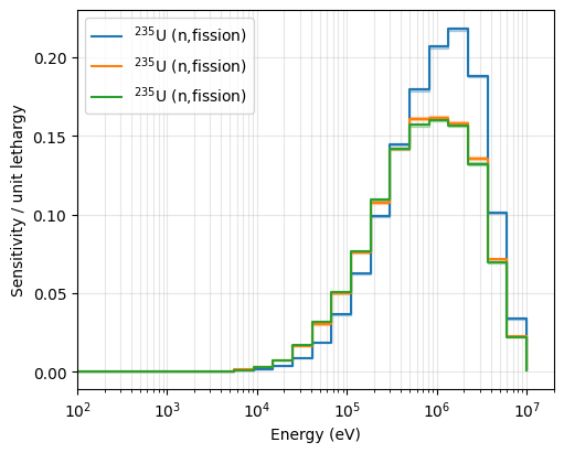
3. Energy-Dependent Sensitivities

Visualizing the sensitivity profiles helps us understand which energy ranges drive the \(k_{\text{eff}}\) response. Below we compare U-235 fission (MT 18) sensitivities across all systems.

zais = [922350]  # U-235
perts = [18]  # Fission (MT 18)

fig, ax = plt.subplots(figsize=(5, 4), layout="constrained")

for benchmark in assimilation_suite.benchmarks:
    benchmark.s.plot_sensitivity(zais=zais, perts=perts, ax=ax)

assimilation_suite.applications["HMF002-002"].s.plot_sensitivity(zais=zais, perts=perts, ax=ax)

ax.set(
    xlim=(1e2, 2e7),
)

C:\Users\dhouben\Documents\andalus\src\andalus\sensitivity.py:230: PerformanceWarning: indexing past lexsort depth may impact performance.
  subset = self.loc[zai, pert]

[(100.0, 20000000.0)]

4. Similarity Analysis (\(c_k\) Index)

The \(c_k\) index quantifies the correlation between systems based on shared nuclear data uncertainties.

\[c_k=\frac{\text{Cov}(1,2)}{\sqrt(\text{Var}(1)\text{Var}(2))}\]

Values close to 1.0 indicate that the benchmark is an excellent surrogate for the application.

# Print the ck-similarity matrix
ck_matrix = assimilation_suite.ck_matrix()
print(ck_matrix)

                HMF001  HMF002-001  HMF002-002
HMF001     1.00000e+00 8.58986e-01 8.61173e-01
HMF002-001 8.58986e-01 1.00000e+00 9.99814e-01
HMF002-002 8.61173e-01 9.99814e-01 1.00000e+00

# Print the ck-similarity values for a specific target
ck_target = assimilation_suite.ck_target("HMF002-002")
print(ck_target)

HMF001       8.61173e-01
HMF002-001   9.99814e-01
Name: HMF002-002, dtype: float64

We can see that HMF002-001 has more than 99% of the nuclear data uncertainties with regards to keff in common, meaning that if we reduce the nuclear data uncertainties in HMF002-001, we will also reduce the uncertainty in predicting keff with regards to the uncertainties due to nuclear data in HMF002-002.

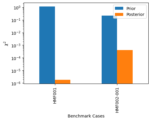
5. Performing the GLLS Adjustment

We now calculate the posterior suite. This updates the nominal values (\(c\)) and reduces the covariance matrix based on the experimental evidence from the benchmarks.

posterior_suite = assimilation_suite.glls()

# Compare Chi-Squared reduction
chi_comparison = pd.DataFrame(
    {
        "Prior": assimilation_suite.individual_chi_squared(nuclear_data=False),
        "Posterior": posterior_suite.individual_chi_squared(nuclear_data=False),
    }
)

fig, ax = plt.subplots(figsize=(5, 4), layout="constrained")

chi_comparison.plot.bar(ax=ax)

ax.set(
    yscale="log",
    ylabel="$\\chi^2$",
    xlabel="Benchmark Cases",
)

plt.show()

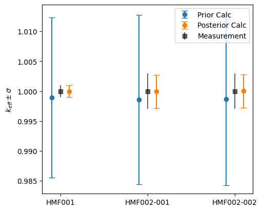
6. Summary of Results

The plot below shows the \(k_{\text{eff}}\) predictions. Note how the Posterior values for the target application (HMF002-002) move significantly closer to the experimental measurement, even though that specific system was not used in the adjustment. This is because HMF002-002 is highly similar to HMF002-001, therefore correcting for the behaviour of one improves the prediction for the behaviour of the other one as well.

prior_unc = assimilation_suite.propagate_nuclear_data_uncertainty()
post_unc = posterior_suite.propagate_nuclear_data_uncertainty()

fig, ax = plt.subplots(figsize=(5, 4), dpi=100, layout="constrained")

x = range(len(assimilation_suite.titles))
ax.errorbar([i - 0.1 for i in x], assimilation_suite.c, yerr=prior_unc, fmt="o", capsize=4, label="Prior Calc")
ax.errorbar([i + 0.1 for i in x], posterior_suite.c, yerr=post_unc, fmt="o", capsize=4, label="Posterior Calc")

# Add experimental measurements (benchmarks + application)
# The final value [1.00000] and uncertainty [0.00300] represent the target application (HMF002-002)
measurement_values = assimilation_suite.benchmarks.m.tolist() + [1.00000]
measurement_uncertainties = assimilation_suite.benchmarks.dm.tolist() + [0.00300]
ax.errorbar(
    x,
    measurement_values,
    yerr=measurement_uncertainties,
    fmt="s",
    color="black",
    label="Measurement",
    alpha=0.6,
)

ax.set_xticks(x)
ax.set_xticklabels(assimilation_suite.titles)
ax.set_ylabel("$k_{eff} \\pm \\sigma$")
ax.legend()
plt.show()