Flux Spectrum and E-Index Analysis

This example demonstrates how to attach a neutron flux spectrum to a Benchmark using a Serpent detector file, visualize it with FluxSpectrum.plot_spectrum, and compute the E-index similarity matrix via AssimilationSuite.e_index_matrix. The E-index quantifies the cosine similarity between sensitivity profiles without the influence of a nuclear data covariance matrix.

1. Setup and Imports

We import andalus for the core logic and matplotlib for visualization.

import matplotlib.pyplot as plt

import andalus

2. Reading Serpent Output

We load the HMF001 (Godiva) benchmark using Benchmark.from_serpent. The optional flux_det argument attaches a FluxSpectrum by reading a named detector from a Serpent _det0.m file. Here we pass the detector name "flux" and the path to the detector output file.

The pertlist filters the sensitivity output to the most physically relevant reactions:

• mt 2 xs: Elastic scattering

• mt 18 xs: Fission

• mt 102 xs: Radiative capture

• nubar prompt: Average prompt neutron multiplicity

• chi prompt: Prompt fission neutron spectrum

hmf001 = andalus.Benchmark.from_serpent(
    title="HMF001",
    m=1.0,
    dm=0.001,
    sens0_path="../data/hmf001.ser_sens0.m",
    results_path="../data/hmf001.ser_res.m",
    pertlist=["mt 2 xs", "mt 18 xs", "mt 102 xs", "nubar prompt", "chi prompt"],
    flux_det=("flux", "../data/hmf001.ser_det0.m"),
)

Reading ../data/hmf001.ser_res.m
WARNING:  SERPENT Serpent 2.2.1 found in ../data/hmf001.ser_res.m, but version 2.1.31 is defined in settings
WARNING:    Attempting to read anyway. Please report strange behaviors/failures to developers.
  - done
Reading ../data/hmf001.ser_sens0.m
  - done
Reading ../data/hmf001.ser_det0.m
  - done

The flux attribute is a FluxSpectrum, a pandas DataFrame subclass with a two-level (E_min_eV, E_max_eV) MultiIndex. We inspect the first few rows to verify the energy grid and flux values.

hmf001.flux.head()

		flux	flux_std
E_min_eV	E_max_eV
0.00001	0.10000	0.000000e+00	0.000000e+00
0.10000	0.54000	0.000000e+00	0.000000e+00
0.54000	4.00000	0.000000e+00	0.000000e+00
4.00000	8.31529	5.409640e-09	5.409640e-09
8.31529	13.70960	0.000000e+00	0.000000e+00

3. Flux Spectrum Characterization

Two scalar metrics summarize where neutrons are most active in energy:

\[\text{EALF} = \exp\!\left(\frac{\sum_i \phi_i \ln \bar{E}_i}{\sum_i \phi_i}\right)\]

\[\langle E \rangle = \frac{\sum_i \phi_i \bar{E}_i}{\sum_i \phi_i}\]

where \(\bar{E}_i = \sqrt{E_{\min,i} \cdot E_{\max,i}}\) is the geometric mean energy of bin \(i\). EALF is the flux-weighted geometric mean (sensitive to the lethargy distribution), while \(\langle E \rangle\) is the flux-weighted arithmetic mean. For a fast spectrum such as HMF001 we expect both to lie well above the thermal region.

print(f"EALF:        {hmf001.flux.ealf:.3e} eV")
print(f"Mean energy: {hmf001.flux.mean_energy:.3e} eV")

EALF:        8.474e+05 eV
Mean energy: 1.461e+06 eV

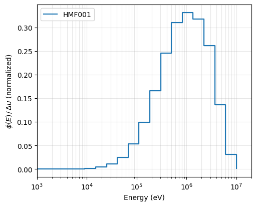
4. Plotting the Flux Spectrum

We plot the normalized flux per unit lethargy, \(\phi(E)/\Delta u\), on a logarithmic energy axis. The shaded band represents the \(1\sigma\) statistical uncertainty from the Serpent tally. The sharp peak in the fast region is characteristic of the bare HEU Godiva configuration.

fig, ax = plt.subplots(figsize=(5, 4), layout="constrained")

hmf001.flux.plot_spectrum(ax=ax)

ax.set(xlim=(1e3, 2e7))

plt.show()

5. E-Index Similarity via AssimilationSuite

The E-index measures the cosine similarity between two sensitivity vectors:

\[E_{ij} = \frac{S_i^T S_j}{\sqrt{S_i^T S_i \cdot S_j^T S_j}}\]

Unlike \(c_k\), the E-index does not involve a covariance matrix, so it captures purely geometric similarity of the sensitivity profiles. We construct a minimal AssimilationSuite with HMF001 as both the benchmark and the application to illustrate the API.

suite = andalus.AssimilationSuite.from_yaml("config.yaml")

Reading ../data/hmf001.ser_res.m
WARNING:  SERPENT Serpent 2.2.1 found in ../data/hmf001.ser_res.m, but version 2.1.31 is defined in settings
WARNING:    Attempting to read anyway. Please report strange behaviors/failures to developers.
  - done
Reading ../data/hmf001.ser_sens0.m
  - done
Reading ../data/hmf002-001.ser_res.m
WARNING:  SERPENT Serpent 2.2.1 found in ../data/hmf002-001.ser_res.m, but version 2.1.31 is defined in settings
WARNING:    Attempting to read anyway. Please report strange behaviors/failures to developers.
  - done
Reading ../data/hmf002-001.ser_sens0.m
  - done
Reading ../data/hmf002-002.ser_res.m
WARNING:  SERPENT Serpent 2.2.1 found in ../data/hmf002-002.ser_res.m, but version 2.1.31 is defined in settings
WARNING:    Attempting to read anyway. Please report strange behaviors/failures to developers.
  - done
Reading ../data/hmf002-002.ser_sens0.m
  - done

e_index = suite.e_index_matrix()
print(e_index)

              HMF001  HMF002-001  HMF002-002
HMF001      1.000000    0.960530    0.957067
HMF002-001  0.960530    1.000000    0.999763
HMF002-002  0.957067    0.999763    1.000000

The diagonal entries equal 1.0 by construction. The off-diagonal value between the benchmark and application reflects how closely aligned their sensitivity profiles are in the multivariate nuclear-data space. An E-index near 1.0 indicates that the two systems are driven by the same energy and reaction dependencies, making the benchmark a strong predictor of the application’s behavior.